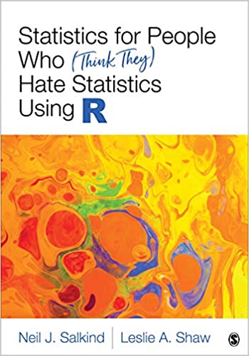
经典教材:爱上统计学Statistics for People Who (think They) Hate Statistics
作者:Neil J. Salkind(1947-2017)
https://www.findagrave.com/memorial/192090437/neil-j-salkind
https://www.socialsciencespace.com/2017/11/gentle-guide-neil-salkind-1947-2017/

The gentle good humor of that answer imbues one of his enduring efforts for SAGE Publishing, the Statistics for People Who (Think They) Hate Statistics books.
“Neil Salkind’s statistics textbooks were so successful because Neil had a unique gift for communicating an often-intimidating subject in a playful and humorous way,” recalled Helen Salmon, a senior acquisitions editor with SAGE. “His bestselling Statistics for People Who (Think They) Hate Statistics put students at ease, without being condescending. Neil was incredibly generous with his time and expertise: he published his email address in the front of his books, and would respond to several emails a day from students from around the world who asked for his advice and help. He was a wonderful author to work with, as he was always dreaming up the next project.”
https://uk.sagepub.com/en-gb/asi/author/neil-joseph-salkind
https://www.amazon.com/Neil-J.-Salkind/e/B000APV1GM
https://www.goodreads.com/author/show/8442.Neil_J_Salkind

Chapter 16: Two Groups Too Many Factors
Import our first data set
ch16ds1<-read.csv('D:/kaiwu_study/study2022love_statistics/16/ch16ds1.csv',header=TRUE,encoding = 'UTF-8')View what we just imported. Did we get what we expected?
head(ch16ds1)Get descriptive statistics about each group
Load the psych library
library(psych)
library(dplyr)
##
## 载入程辑包:'dplyr'## The following objects are masked from 'package:stats':
##
## filter, lag## The following objects are masked from 'package:base':
##
## intersect, setdiff, setequal, unionlibrary(ggplot2)##
## 载入程辑包:'ggplot2'## The following objects are masked from 'package:psych':
##
## %+%, alphalibrary(car)## 载入需要的程辑包:carData##
## 载入程辑包:'car'## The following object is masked from 'package:dplyr':
##
## recode## The following object is masked from 'package:psych':
##
## logitUse the function
summary(ch16ds1)## Treatment Gender Loss
## Length:40 Length:40 Min. :54.00
## Class :character Class :character 1st Qu.:65.00
## Mode :character Mode :character Median :76.00
## Mean :73.97
## 3rd Qu.:78.25
## Max. :98.00describeBy(ch16ds1$Loss, group = list(ch16ds1$Treatment,
ch16ds1$Gender))##
## Descriptive statistics by group
## : High Impact
## : Female
## vars n mean sd median trimmed mad min max range skew kurtosis se
## X1 1 10 79.4 11.89 84.5 79.88 8.15 65 90 25 -0.23 -2 3.76
## ------------------------------------------------------------
## : Low Impact
## : Female
## vars n mean sd median trimmed mad min max range skew kurtosis se
## X1 1 10 64 11.23 60.5 62.38 9.64 54 87 33 0.81 -0.8 3.55
## ------------------------------------------------------------
## : High Impact
## : Male
## vars n mean sd median trimmed mad min max range skew kurtosis se
## X1 1 10 73.7 6.67 76 75.5 0 55 78 23 -2.15 3.21 2.11
## ------------------------------------------------------------
## : Low Impact
## : Male
## vars n mean sd median trimmed mad min max range skew kurtosis se
## X1 1 10 78.8 11.04 76 79.25 1.48 56 98 42 -0.25 -0.17 3.49ch16ds1sumary<- ch16ds1 %>%
group_by(Treatment, Gender) %>%
summarize(n = n(),
mean = mean(Loss),
sd = sd(Loss),
ci = qt(0.975, df = n - 1)* sd /sqrt(n))## `summarise()` has grouped output by 'Treatment'. You can override using the
## `.groups` argument.ch16ds1sumaryRun the ANOVA
# Check the default contrasts used by aov
options("contrasts")
## $contrasts
## unordered ordered
## "contr.treatment" "contr.poly"# Change the default for categorical variables
options(contrasts = c("contr.helmert", "contr.poly"))
# Check the contrasts again to make sure it worked
options("contrasts")## $contrasts
## [1] "contr.helmert" "contr.poly"Calculate your ANOVA
m1 <- aov(Loss ~ Treatment + Gender + Treatment*Gender, data = ch16ds1)Look at the results from the ANOVA
summary(m1)## Df Sum Sq Mean Sq F value Pr(>F)
## Treatment 1 265 265.2 2.444 0.12669
## Gender 1 207 207.0 1.908 0.17570
## Treatment:Gender 1 1051 1050.6 9.683 0.00363 **
## Residuals 36 3906 108.5
## ---
## Signif. codes: 0 '***' 0.001 '**' 0.01 '*' 0.05 '.' 0.1 ' ' 1Look at the results
Anova(m1, type = 3)Check the homogeneity of variance assumption
leveneTest(Loss ~ Treatment*Gender, data = ch16ds1)Draw an interaction plot
interaction.plot(x.factor = ch16ds1$Treatment,
                 trace.factor = ch16ds1$Gender,
                 response = ch16ds1$Loss)
interaction.plot(x.factor = ch16ds1$Treatment,
trace.factor = ch16ds1$Gender,
response = ch16ds1$Loss,
fixed = TRUE,
leg.bty = "b",
xlab = "Treatment",
ylab = "Weight Loss",
trace.label = "Gender",
ylim = c(60, 85))library(HH)## 载入需要的程辑包:lattice## 载入需要的程辑包:grid## 载入需要的程辑包:latticeExtra##
## 载入程辑包:'latticeExtra'## The following object is masked from 'package:ggplot2':
##
## layer## 载入需要的程辑包:multcomp## 载入需要的程辑包:mvtnorm## 载入需要的程辑包:survival## 载入需要的程辑包:TH.data## 载入需要的程辑包:MASS##
## 载入程辑包:'MASS'## The following object is masked from 'package:dplyr':
##
## select##
## 载入程辑包:'TH.data'## The following object is masked from 'package:MASS':
##
## geyser## 载入需要的程辑包:gridExtra##
## 载入程辑包:'gridExtra'## The following object is masked from 'package:dplyr':
##
## combine##
## 载入程辑包:'HH'## The following objects are masked from 'package:car':
##
## logit, vif## The following object is masked from 'package:psych':
##
## logitinteraction2wt(data= ch16ds1,Loss~Treatment*Gender)Compare the pairs of groups
TukeyHSD(m1)## Tukey multiple comparisons of means
## 95% family-wise confidence level
##
## Fit: aov(formula = Loss ~ Treatment + Gender + Treatment * Gender, data = ch16ds1)
##
## $Treatment
## diff lwr upr p adj
## Low Impact-High Impact -5.15 -11.83049 1.530493 0.1266935
##
## $Gender
## diff lwr upr p adj
## Male-Female 4.55 -2.130493 11.23049 0.1756979
##
## $`Treatment:Gender`
## diff lwr upr p adj
## Low Impact:Female-High Impact:Female -15.4 -27.94609 -2.85391 0.0110583
## High Impact:Male-High Impact:Female -5.7 -18.24609 6.84609 0.6162344
## Low Impact:Male-High Impact:Female -0.6 -13.14609 11.94609 0.9992219
## High Impact:Male-Low Impact:Female 9.7 -2.84609 22.24609 0.1782508
## Low Impact:Male-Low Impact:Female 14.8 2.25391 27.34609 0.0154282
## Low Impact:Male-High Impact:Male 5.1 -7.44609 17.64609 0.6949307
