- 文章信息
- 作者: kaiwu
- 点击数:391
https://www.forbeginnersbooks.com/
https://en.wikipedia.org/wiki/For_Beginners
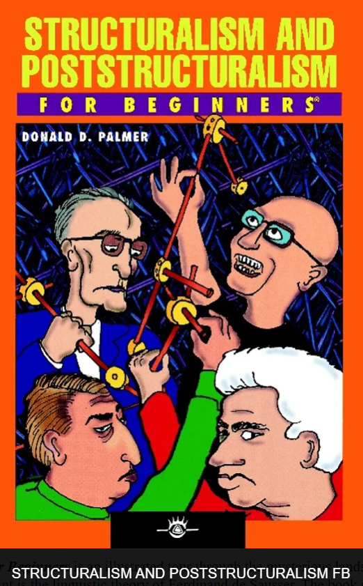
The For Beginners series was launched in the mid-1970s, but became out of print and often unavailable after the 2001 death of co-founder and publisher Glenn Thompson. In 2007, a consortium of investors revived the series, reprinted back issues, and promised to publish between six and nine new issues each year. The current publisher is Dawn Reshen-Doty.


- 文章信息
- 作者: kaiwu
- 点击数:678
The servitization in manufacturing may be the most important feature of Industry 4.0
http://kaiwu.city/joomla/index.php/83-job-ai
1.The future of employment
http://kaiwu.city/index.php/job-ai
Frey, C. B., & Osborne, M. A. (2017). The future of employment: How susceptible are jobs to computerisation? Technological Forecasting and Social Change, 114, 254–280.
http://dx.doi.org/10.1016/j.techfore.2016.08.019
https://www.sciencedirect.com/science/article/pii/S0040162516302244
https://www.oxfordmartin.ox.ac.uk/downloads/academic/The_Future_of_Employment.pdf
The future of employment
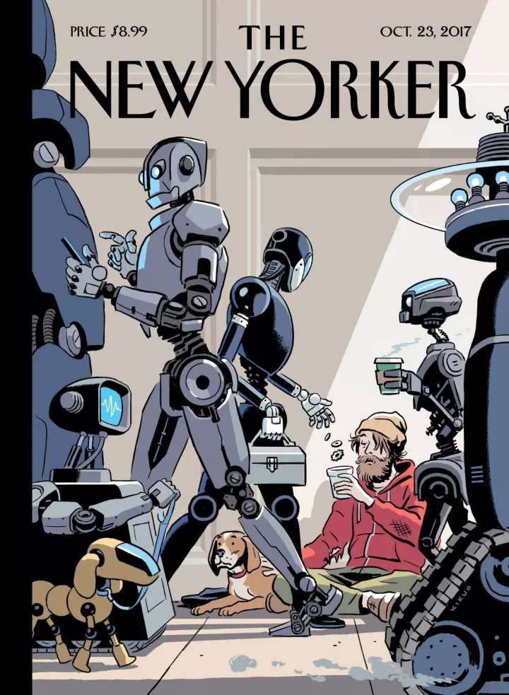
“Tech Support” by R. Kikuo Johnson.
《NewYorker》https://www.newyorker.com/culture/cover-story/cover-story-2017-10-23
https://www.npr.org/sections/money/2015/05/21/408234543/will-your-job-be-done-by-a-machine
2.Robot made of magnetic slime could grab objects inside your body
Wilkins, A. (2022, March 21). Robot Made of Magnetic Slime Could Grab Objects Inside Your Body. New Scientist. https://www.newscientist.com/article/2314395-robot-made-of-magnetic-slime-could-grab-objects-inside-your-body/
3.robot restaurant in Dalian
大连人工智能基地科学餐厅(万达公寓店)
4.Restaurant of the Future 2023 | Food Robots On The Rise
https://www.youtube.com/watch?v=KQkmFZQ-2SA
5.Betop 博涛公司
https://www.betoptech.com/index.html
A.I. teaches itself to drive in Trackmania
https://www.bilibili.com/video/BV1GS4y1Y77r
https://www.youtube.com/watch?v=a8Bo2DHrrow
The inside story of ChatGPT's astonishing potential
https://www.ted.com/talks/greg_brockman_the_inside_story_of_chatgpt_s_astonishing_potential/c
https://www.bilibili.com/video/BV1NM411P7zj/
what is the difference between objective authenticity and existential authenticity in tourism experience?
what is artificial intelligence?
can you summarize the five features of artificial intelligence?
how to transform json file into csv using python?
panda is studying for final exam
https://www.dedao.cn/course/detail?id=v12pOMZN7mbJwgMsbpJDrjxdYaGkoE
NFT Explained In 5 Minutes | What Is NFT?
https://www.youtube.com/watch?v=NNQLJcJEzv0
NFT Explained In 4 Minutes
https://www.bilibili.com/video/BV1SB4y1e79W/
Rashideh, W. (2020). Blockchain technology framework: Current and future perspectives for the tourism industry. Tourism Management, 80, 104125. https://doi.org/10.1016/j.tourman.2020.104125
Flecha-Barrio, M. D., Palomo, J., Figueroa-Domecq, C., & Segovia-Perez, M. (2020). Blockchain Implementation in Hotel Management. In J. Neidhardt & W. Wörndl , Information and Communication Technologies in Tourism 2020 (pp. 255–266). Springer International Publishing. https://doi.org/10.1007/978-3-030-36737-4_21
The Metaverse and How We'll Build It Together -- Connect 2021
https://www.youtube.com/watch?v=Uvufun6xer8
https://www.bilibili.com/video/BV1qb4y1q77u
https://www.wired.com/story/what-is-the-metaverse/
https://news.berkeley.edu/2020/05/16/watch-blockeley-uc-berkeleys-online-minecraft-commencement/
https://artsandculture.google.com/
https://artsandculture.google.com/story/WgUx5YGDnc6MzQ
https://artsandculture.google.com/asset/the-starry-night-vincent-van-gogh/bgEuwDxel93-Pg
http://tour.quanjingke.com/xiangmu/songdugucheng/5qingmingshangheyuan/tour.html
Gursoy, D., Malodia, S., & Dhir, A. (2022). The Metaverse in the Hospitality and Tourism Industry: An Overview of Current Trends and Future Research Directions. Journal of Hospitality Marketing & Management, 0(0), 1–8. https://doi.org/10.1080/19368623.2022.2072504
Han, D.-I. D., Bergs, Y., & Moorhouse, N. (2022). Virtual Reality Consumer Experience Escapes: Preparing for the Metaverse. Virtual Reality. https://doi.org/10.1007/s10055-022-00641-7
Kozinets, R. V. (2022). Immersive Netnography: A Novel Method for Service Experience Research in Virtual Reality, Augmented Reality and Metaverse Contexts. Journal of Service Management,. https://doi.org/10.1108/JOSM-12-2021-0481
- 文章信息
- 作者: kaiwu
- 点击数:709
https://mp.weixin.qq.com/s/BXou7IVHkPBztfjFOIJMSQ


Institute for Dark Tourism Research (iDTR). University of Central Lancashire. Retrieved April 11, 2023, from https://www.uclan.ac.uk/research/activity/dark-tourism
You and Yours—Digital wallets, dark tourism, and tackling insurance fraud—BBC Sounds. (n.d.). Retrieved April 11, 2023, from https://www.bbc.co.uk/sounds/play/b01gvvxp
- Allman, H. R. (2017). Motivations and Intentions of Tourists to Visit Dark Tourism Locations [Doctoral dissertation, Iowa State University]. In ProQuest Dissertations and Theses. https://www.proquest.com/docview/1918165601/abstract/2FF6072A15854BD4PQ/11
- Biran, A., & Hyde, K. F. (2013). New Perspectives on Dark Tourism. International Journal of Culture, Tourism and Hospitality Research, 7(3), 191–198. https://doi.org/10.1108/IJCTHR-05-2013-0032
- Campbell-Firkus, D. D. (2021). The Stories We Tell: Expanding Conceptions of Dark Tourism and Cultural Identity in America [Master’s thesis, Middle Tennessee State University]. In ProQuest Dissertations and Theses. https://jewlscholar.mtsu.edu/items/49119caa-bf49-49e2-bcfa-d9ef1b2a3a8b/full
- Dresler, E. (2023). Multiplicity of Moral Emotions in Educational Dark Tourism. Tourism Management Perspectives, 46, 101094. https://doi.org/10.1016/j.tmp.2023.101094
- Filep, S., Laing, J., & Csikszentmihalyi, M. (2019). Positive tourism. Routledge.
- Frew, E. (Ed.). (2016). Dark Tourism and Place Identity: Managing and Interpreting Dark Places. Routledge. https://www.taylorfrancis.com/books/edit/10.4324/9780203134900/dark-tourism-place-identity-leanne-white-elspeth-frew
- Hohenhaus, P. (2021). Atlas of Dark Destinations: Explore the World of Dark Tourism. Laurence King Publishing.
- Kerr, M. M. (Ed.). (2022). Children, Young People and Dark Tourism. Routledge.
- Lennon, J. (2017). Dark Tourism. In J. Lennon, Oxford Research Encyclopedia of Criminology and Criminal Justice. Oxford University Press. https://doi.org/10.1093/acrefore/9780190264079.013.212
- Lennon, J. J., & Foley, M. (2000). Dark Tourism. Continuum.
- Light, D. (2017). Progress in Dark Tourism and Thanatourism Research: An Uneasy Relationship with Heritage Tourism. Tourism Management, 61, 275–301. https://doi.org/10.1016/j.tourman.2017.01.011
- Luna-Cortés, G., López-Bonilla, L. M., & López-Bonilla, J. M. (2022). The Consumption of Dark Narratives: A Systematic Review and Research Agenda. Journal of Business Research, 145, 524–534. https://doi.org/10.1016/j.jbusres.2022.03.013
- Lv, X., Lu, R., Xu, S., Sun, J., & Yang, Y. (2022). Exploring Visual Embodiment Effect in Dark Tourism: The Influence of Visual Darkness on Dark Experience. Tourism Management, 89, 104438. https://doi.org/10.1016/j.tourman.2021.104438
- Lv, X., Luo, H., Xu, S., Sun, J., Lu, R., & Hu, Y. (2022). Dark Tourism Spectrum: Visual Expression of Dark Experience. Tourism Management, 93, 104580. https://doi.org/10.1016/j.tourman.2022.104580
- MacAmhalai, M. (2009). The Dialectics of Dark Tourism [Doctoral dissertation, University of Ulster (United Kingdom)]. In PQDT - UK & Ireland. https://ethos.bl.uk/OrderDetails.do?uin=uk.bl.ethos.510462
- Magano, J., Fraiz-Brea, J. A., & Ângela Leite. (2023). Dark Tourism, the Holocaust, and Well-Being: A Systematic Review. Heliyon, 9(1), e13064. https://doi.org/10.1016/j.heliyon.2023.e13064
- Martini, A., & Buda, D. M. (2020). Dark Tourism and Affect: Framing Places of Death and Disaster. Current Issues in Tourism, 23(6), 679–692. https://doi.org/10.1080/13683500.2018.1518972
- McDaniel, K. N. (Ed.). (2018). Virtual Dark Tourism: Ghost Roads. Palgrave Macmillan. https://doi.org/10.1007/978-3-319-74687-6
- Mitchell, V., Henthorne, T. L., & George, B. (2020). Making Sense of Dark Tourism: Typologies, Motivations and Future Development of Theory. In M. E. Korstanje & H. Seraphin, Tourism, Terrorism and Security (pp. 103–114). Emerald Publishing Limited. https://doi.org/10.1108/978-1-83867-905-720201007
- Olsen, D. H., & C.A.B. International (2019). Dark Tourism and Pilgrimage. CABI.
- Pastor, D. (2023). Tourism and Memory: Visitor Experiences of the Nazi and Gdr Past . Routledge.
- Poade, D. M. (2017). The Business of “Dark Tourism”: The Management of “Dark Tourism” Visitor Sites and Attractions, with Special Reference to Innovation [Doctoral dissertation, University of Exeter (United Kingdom)]. In PQDT - UK & Ireland. https://ore.exeter.ac.uk/repository/handle/10871/28820
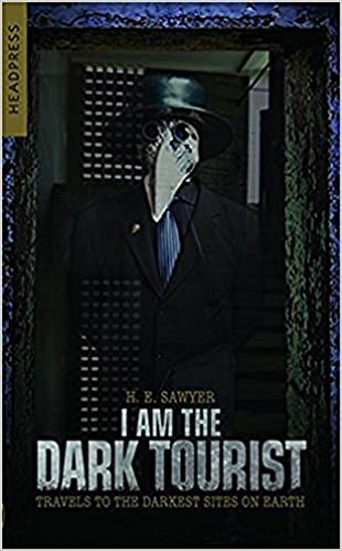
- Sawyer, H. E. (2018). I Am The Dark Tourist: Travels to the Darkest Sites on Earth. Headpress.
- Sirisena, H. (2021). Dark Tourist: Essays. Mad Creek Books.
- Stone, P. (2013). Dark Tourism Scholarship: A Critical Review. International Journal of Culture, Tourism and Hospitality Research, 7(3), 307–318. https://doi.org/10.1108/IJCTHR-06-2013-0039
- Stone, P. R. (2011). Death, Dying and Dark Tourism in Contemporary Society: A Theoretical and Empirical Analysis [Doctoral dissertation, University of Central Lancashire (United Kingdom)]. In PQDT - UK & Ireland. https://clok.uclan.ac.uk/1870/1/StonePPhD_thesis_final.pdf
- Stone, P. R., Hartmann, R., Seaton, A. V., Sharpley, R., & White, L. (2018). The Palgrave Handbook of Dark Tourism Studies. Palgrave Macmillan. https://link.springer.com/book/10.1057/978-1-137-47566-4
- Stone, P., & Sharpley, R. (2008). Consuming Dark Tourism: A Thanatological Perspective. Annals of Tourism Research, 35(2), 574–595. https://doi.org/10.1016/j.annals.2008.02.003
-
Stone, P. R. (2006). A Dark Tourism Spectrum: Towards a Typology of Death and Macabre Related Tourist Sites, Attractions and Exhibitions. Tourism: An International Interdisciplinary Journal, 54(2), 145–160.
-
Stone, P. R. (2012). Dark Tourism and Significant Other Death: Towards a Model of Mortality Mediation. Annals of Tourism Research, 39(3), 1565–1587. https://doi.org/10.1016/j.annals.2012.04.007
-
Storey, A., Nurse, A., Sergi, A., Lloyd, A., Colliver, B., Ancrum, C., Rusu, D., Wilson, D., Yates, D., Frankis, D. J., Carrabine, E., Smith, E., Winlow, E., Buck-Matthews, E., Potter, G., Gallacher, G., London, H., Cook, I. R., Richards, J., … Laverick, W. (2023). 50 Dark Destinations: Crime and Contemporary Tourism. Policy Press.
- Šuligoj, M., & Kennell, J. (2022). The Role of Dark Commemorative and Sport Events in Peaceful Coexistence in the Western Balkans. Journal of Sustainable Tourism, 30(2–3), 408–426. https://doi.org/10.1080/09669582.2021.1938090
- Thapa Magar, A. (2018). Enlightening Dark Tourism in Nepal [Master’s thesis, University of North Texas]. In ProQuest Dissertations and Theses. https://www.proquest.com/docview/2191733971/abstract/2FF6072A15854BD4PQ/3
-
Tzanelli, R. (2018). Schematising Hospitality: Ai Weiwei’s Activist Artwork as a Form of Dark Travel. Mobilities, 13(4), 520–534. https://doi.org/10.1080/17450101.2017.1411817
- Wang, J., Chang, M., Luo, X., Qiu, R., & Zou, T. (2023). How Perceived Authenticity Affects Tourist Satisfaction and Behavioral Intention Towards Natural Disaster Memorials: A Mediation Analysis. Tourism Management Perspectives, 46, 101085. https://doi.org/10.1016/j.tmp.2023.101085
- Willis, E. (2014). Theatricality, Dark Tourism and Ethical Spectatorship: Absent Others. Palgrave Macmillan UK. http://gen.lib.rus.ec/book/index.php?md5=2cd30fd56c14a530cc0c3a37728345a3
- Wyatt, B., Leask, A., & Barron, P. (2021). Designing Dark Tourism Experiences: An Exploration of Edutainment Interpretation at Lighter Dark Visitor Attractions. Journal of Heritage Tourism, 16(4), 433–449. https://doi.org/10.1080/1743873X.2020.1858087
- Wyatt, B., Leask, A., & Barron, P. (2023). Re-Enactment in Lighter Dark Tourism: An Exploration of Re-Enactor Tour Guides and Their Perspectives on Creating Visitor Experiences. Journal of Travel Research, 00472875221151074. https://doi.org/10.1177/00472875221151074
- Yan, B.-J., Zhang, J., Zhang, H.-L., Lu, S.-J., & Guo, Y.-R. (2016). Investigating the Motivation–Experience Relationship in a Dark Tourism Space: A Case Study of the Beichuan Earthquake Relics, China. Tourism Management, 53, 108–121. https://doi.org/10.1016/j.tourman.2015.09.014
- Zhang, Y. (2022). Experiencing Human Identity at Dark Tourism Sites of Natural Disasters. Tourism Management, 89, 104451. https://doi.org/10.1016/j.tourman.2021.104451
- 周永博. (2020). 黑色叙事对旅游目的地引致形象的影响机制. 旅游学刊, 35(2), 65–79. https://doi.org/10.19765/j.cnki.1002-5006.2020.02.010
- 孙佼佼. (2018). 黑色旅游体验的心理机制与目的地的意义再表征 [博士, 东北财经大学]. https://kns.cnki.net/kcms2/article/abstract?v=3uoqIhG8C447WN1SO36whLpCgh0R0Z-iDdIt-WSAdV5IJ_Uy2HKRAbgS6zJ0wMCTJ4muPbQP-xXdExlKluCzZVT-mZYBMSaV&uniplatform=NZKPT
- 李经龙、蒋韶檀. (2022). 中国黑色旅游研究进展——基于CiteSpace的文献计量分析. 旅游导刊, 6(6), 76–96.
- 王金伟、张赛茵. (2016). 灾害纪念地的黑色旅游者:动机、类型化及其差异——以北川地震遗址区为例. 地理研究, 35(8), 1576–1588.
- 王金伟, 杨佳旭, 郑春晖, & 王琛琛. (2019). 黑色旅游地游客动机对目的地形象的影响研究——以北川地震遗址区为例. 旅游学刊, 34(9), 114–126. https://doi.org/10.19765/j.cnki.1002-5006.2019.09.015
- 王金伟、段冰杰. (2021). Dark Tourism学术研究:进展与展望. 旅游科学, 35(5), 81–103. https://doi.org/10.16323/j.cnki.lykx.2021.05.006
- 谢伶、王金伟、吕杰华. (2019). 国际黑色旅游研究的知识图谱——基于CiteSpace的计量分析. 资源科学, 41(3), 454–466.
- 谢彦君、孙佼佼. (2016). 黑色旅游的愉悦情感与美丑双重体验. 财经问题研究, 3, 116–122.
- 谢彦君、 孙佼佼、卫银栋. (2015). 论黑色旅游的愉悦性:一种体验视角下的死亡观照. 旅游学刊, 30(3), 86–94.
- 鲁瑞华. (2022). 见墨者黑?视觉“黑”对黑色旅游体验的影响研究 [硕士, 西南财经大学]. https://doi.org/10.27412/d.cnki.gxncu.2022.001683
- 文章信息
- 作者: kaiwu
- 点击数:812
![]()
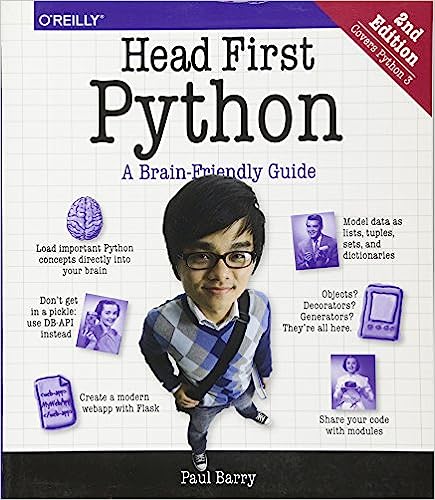
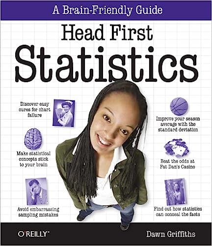
O’Reilly出版社的head first(深入浅出)系列书籍以特殊的方式排版,整合大量的图片和有趣的内容,提供符合直觉的理解方式,让学习自然而有趣,有利于客服恐惧心理和畏难情绪,非常适合初学者使用,。
https://book.douban.com/series/10044
head first书系(55本)


https://wiki.alquds.edu/?query=Head_First_(book_series)
Head First is a series of introductory instructional books to many topics, published by O'Reilly Media. It stresses an unorthodox, visually intensive, reader-involving combination of puzzles, jokes, nonstandard design and layout, and an engaging, conversational style to immerse the reader in a given topic.
Originally, the series covered programming and software engineering, but is now expanding to other topics in science, mathematics and business, due to success. The series was created by Bert Bates and Kathy Sierra, and began with Head First Java in 2003.
https://www.thriftbooks.com/series/head-first-series/37364
https://www.amazon.com/b?node=15123901011
https://book.douban.com/series/4033