
- 文章信息
- 作者: kaiwu
- 点击数:510
https://www.ibm.com/cn-zh/topics/generative-ai
生成式 AI(generative artificial inteligence),有时也称作 gen AI,是一种人工智能 (AI),能够创建原创内容(例如文本、图像、视频、音频或软件代码)以响应用户的提示或请求。
1. transform 模型
经典论文
Vaswani, A., Shazeer, N., Parmar, N., Uszkoreit, J., Jones, L., Gomez, A. N., Kaiser, L., & Polosukhin, I. (2017). Attention Is All You Need (arXiv:1706.03762). arXiv. https://doi.org/10.48550/arXiv.1706.03762
视频解读
https://www.bilibili.com/video/BV1gG411a7bw/
科技参考解读
https://www.dedao.cn/course/article?id=3bezDG7wBonmJwgeE9JvQkAg5PyO1x
2.国际网站
2.1 chatGPT from openAI
2.2 gemini from google
2.3 claude from anthropic
https://www.anthropic.com/claude
2.4 llama from meta
https://llama.meta.com/llama3/
3.国内网站
3.1 秘塔metaso
3.2 月之暗面kimi
3.3 文心一言(baidu.com)
3.4 通义千问 (阿里云)
3.5 讯飞星火(科大讯飞公司iflytek)
3.6 元宝AI(腾讯)
3.7 豆包AI(字节跳动)
3.8 音乐创作suno

4.具体练习
4.1 检索问题
检索短语:旅游体验的本真性问题
检索短语:什么是旅游体验中的建构主义本真?请举出5个例子
4.2 检索代码
检索短语:如何用python导入json数据
检索短语:如何把导入的数据另存为feather格式
4.3 总结文稿
Wang, N. (1999). Rethinking Authenticity in Tourism Experience. Annals of Tourism Research, 26(2), 349–370. https://doi.org/10.1016/S0160-7383(98)00103-0
英文论文全文下载:
http://kaiwu.city/openfiles/rethinking_authenticity1999wang_ning.pdf
短语:请用200字总结一下这个文件
短语:请列出小标题,从6个方面总结一下这个文件
短语:请从5个方面比较一下建构主义本真(Constructive authenticity)与存在主义本真(Existential authenticity)的区别
短语:请从5个方面,比较一下reality、authenticity、originality这3个词的区别和联系
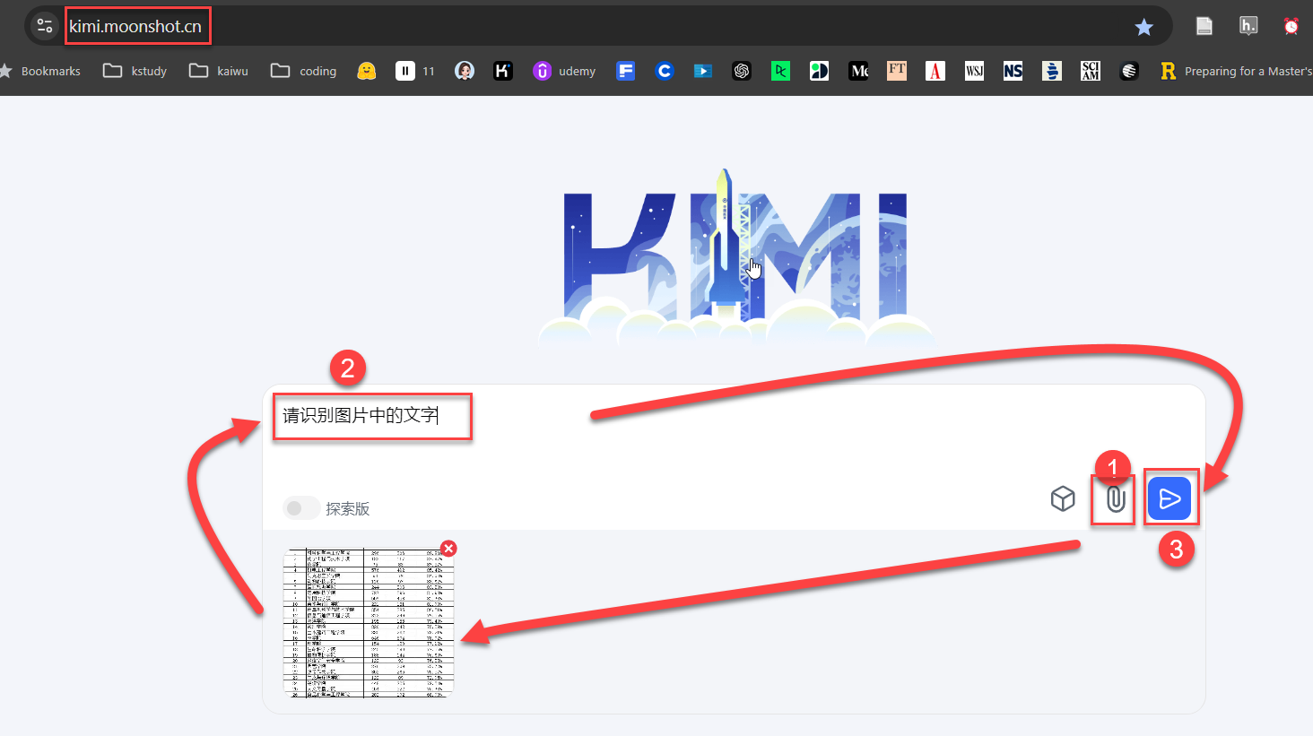
4.4 OCR识别

GAI平台:
doubao AI
或
KIMI
短语:请识别为文字,并用表格整理一下
4.5 翻译
短语:推迟2天,周六下午两点来我办公室讨论一下,请翻译为英文
短语:请提供8个版本
短语:Happiness through vacationing: Just a temporary boost or long-term benefits,请翻译为中文
短语:Although the potentialities of artificial intelligence (AI) are motivating its fast integration in organizations, our knowledge on how to capture organizational value out of these investments is still scarce. Relying on an approach to dynamic capabilities that focuses on the team level, we examine how humans and AI create interactions that engage both agents in productive dialogue for value co-creation. Our analysis is based on a longitudinal case of the development of a recruitment algorithm at a national subsidiary of Santander bank. Our results allow to identify three main sets of human-AI teaming interactions: achieving interoperability, building trust, and producing mutual knowledge gains. We elaborate a set of propositions on how the value of AI is increased when such interactions are created through productive dialogue, opening the scope for further research on the teaming dynamics that turn the collaboration between both agents into a source of value creation for companie. 请翻译为中文
这段话来自论文的摘要:
4.6 诗歌
短语:请依据《水调歌头》词牌,做出一首词,关于大学生春天郊游
短语:注意押韵,使用安、然,an这种韵脚
4.7 数据分析
(1)示例数据集 (tourist satisfaction)

调查问卷
![]() http://kaiwu.city/openfiles/tourist_satisfaction_questionnaire_cn.pdf
http://kaiwu.city/openfiles/tourist_satisfaction_questionnaire_cn.pdf
No. 变量名 变量名标签
1 sid 编号
2 gender 性别
3 byear 出生年份
4 region 区域
5 income 月收入
6 expense 旅游支出
7 type3 旅游目的地类型
8 type2 旅游活动类型
9 thotel 酒店类型
10 sat1 景区sat
11 sat2 住宿sat
12 sat3 餐饮sat
13 sat4 交通sat
14 sat5 娱乐sat
15 sat6 购物sat
16 ri1 评论数量imp
17 ri2 评论的发表日期imp
18 ri3 评论相关性imp
19 ri4 评论中的正向评价imp
20 ri5 评论发布者的资信度imp
21 rp1 评论数量per
22 rp2 评论的发表日期per
23 rp3 评论相关性per
24 rp4 评论中的正向评价per
25 rp5 评论发布者的资信度per
26 te1 刺激感
27 te2 活动偏好
28 te3 旅游经历
29 te4 兴奋感
30 te5 寻求解放
31 te6 自由感
32 te7 新鲜
33 te8 恢复
34 zh1 人多不自在
35 zh2 不喜欢人际交往
36 zh3 不擅长人际交往
37 zh4 避免与人直接交流
38 zh5 外出很累
39 zh6 尽量不外出
40 zh7 外出麻烦
41 latitude 纬度
42 longitude 经度
Value labels gender
1 男
2 女.
Value labels region
1 华中
2 华东
3 华北
4 东北
5 西北
6 西南
7 华西.
Value labels type3
1 自然风光类型
2 历史文化类型
3 自然风光与历史文化混合的类型.
Value labels type2
1 观赏型
2 参与型.
Value labels thotel
1 经济型酒店
2 豪华型酒店
3 民宿
4 酒店式公寓.
(2)通用数据格式 (没有 variable labels变量名标签和 value labels变量值标签)
 http://kaiwu.city/openfiles/tourist.csv
短语:请总结一下这个数据集
短语:请提供对性别gender变量进行频数分析的python代码
4.8 TTS (text to speech)
![]()
----
https://en.wikipedia.org/wiki/Generative_artificial_intelligence
Generative artificial intelligence (generative AI, GenAI, or GAI) is artificial intelligence capable of generating text, images, videos, or other data using generative models, often in response to prompts. Generative AI models learn the patterns and structure of their input training data and then generate new data that has similar characteristics.
4.9 创作歌曲
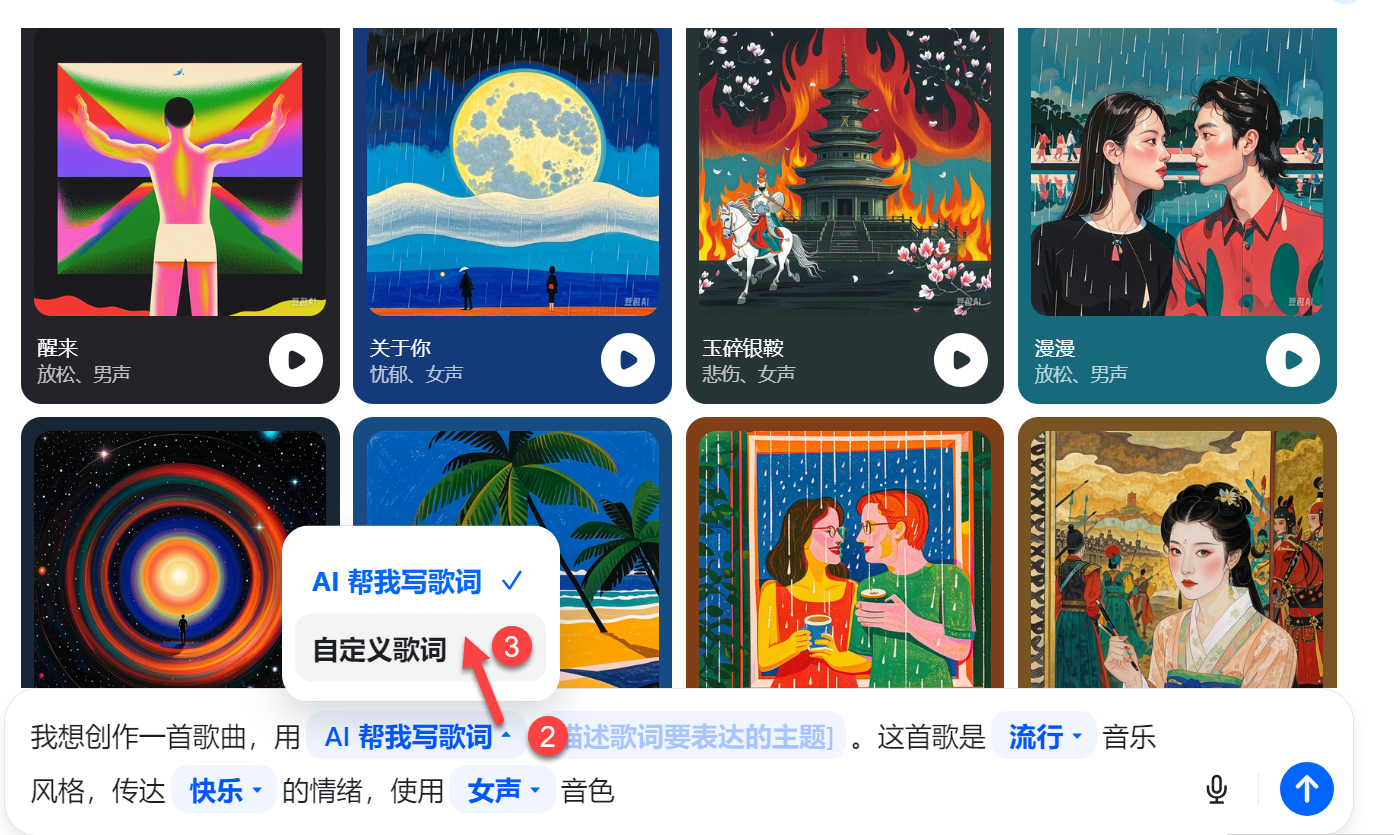
短语:我想创作一首歌曲,用【自定义歌词】,这首歌是【摇滚】音乐风格,传达【兴奋】的情绪,使用【男声】音色。
自定义歌词:再别康桥,徐志摩
4.10 生成图片
短语:请生成一张图片,1个女孩早晨在海边跑步,身着红色T恤,扎马尾辫,海里面有小岛,天上有海鸥,可以看到朝霞。

短语:请生成一张图片,漫画风格,场景是酒店的大堂,展现人工智能对酒店的影响,要有员工、顾客、机器人。


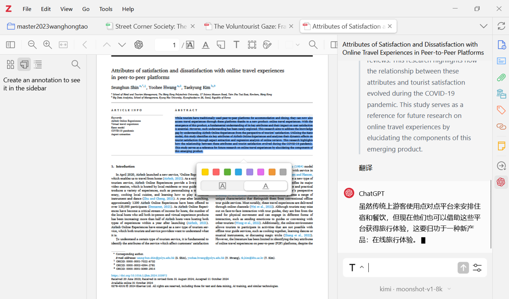
4.11 zotero整合AI
文献管理软件zotero
http://kaiwu.city/index.php/zotero
![]()
ZOTERO(http://www.zotero.org/)是美国乔治梅森大学历史与传播中心提供的免费开源软件,是目前功能最强大、最为流行的一款文献管理软件,绝大多数欧美大学图书馆都提供ZOTERO使用有关的简介。
https://www.bilibili.com/video/BV1zBpUeDEzM/
https://zotero-chinese.com/user-guide/plugins/zotero-gpt.html
https://github.com/MuiseDestiny/zotero-gpt
https://platform.moonshot.cn/console/account
4.12 AI与管理科学(运筹学)
http://kaiwu.city/index.php/solver
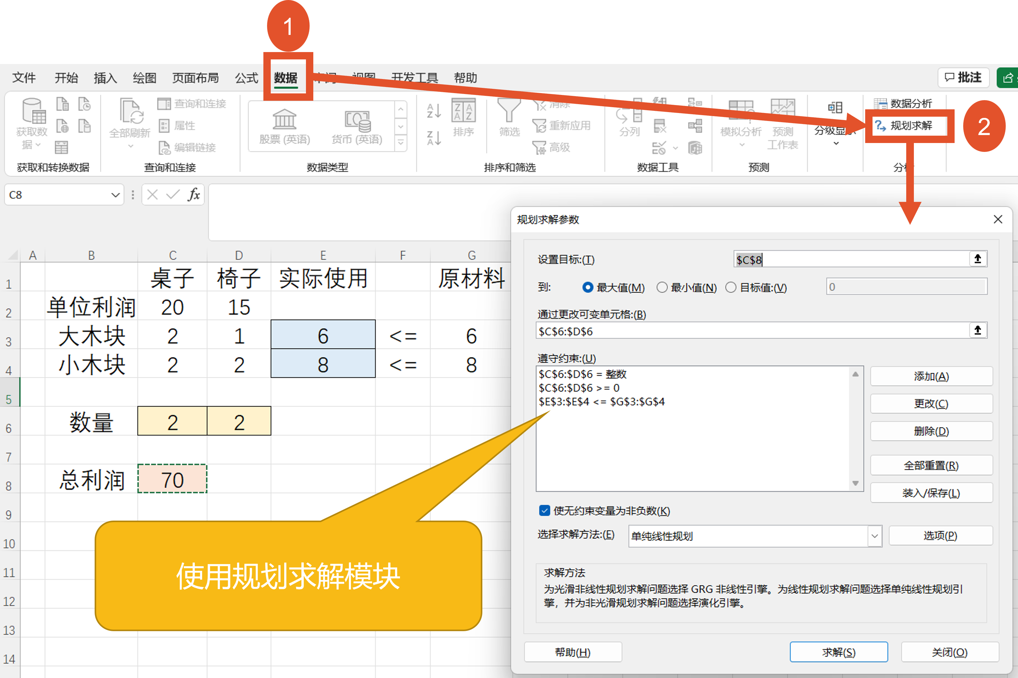
每个小组有 8个小木块和6 个大木块) ,
每张桌子需要2个大木块和2个小木块,
每把椅子需要1个大木块和2个小木块,
拼出1张桌子计20分,拼出1把椅子记15分,
问拼几张桌子、几把椅子,使总得分最高?
5.本地(无需联网)运行大语言模型LLaMa
http://kaiwu.city/index.php/ollama

- 文章信息
- 作者: kaiwu
- 点击数:133
1.关于示例数据集 (tourist satisfaction)
1.1调查问卷
![]() http://kaiwu.city/openfiles/tourist_satisfaction_questionnaire_cn.pdf
http://kaiwu.city/openfiles/tourist_satisfaction_questionnaire_cn.pdf
| No. | 变量名 | 变量名标签 |
| 1 | sid | 编号 |
| 2 | gender | 性别 |
| 3 | byear | 出生年份 |
| 4 | region | 区域 |
| 5 | income | 月收入 |
| 6 | expense | 旅游支出 |
| 7 | type3 | 旅游目的地类型 |
| 8 | type2 | 旅游活动类型 |
| 9 | thotel | 酒店类型 |
| 10 | sat1 | 景区sat |
| 11 | sat2 | 住宿sat |
| 12 | sat3 | 餐饮sat |
| 13 | sat4 | 交通sat |
| 14 | sat5 | 娱乐sat |
| 15 | sat6 | 购物sat |
| 16 | ri1 | 评论数量imp |
| 17 | ri2 | 评论的发表日期imp |
| 18 | ri3 | 评论相关性imp |
| 19 | ri4 | 评论中的正向评价imp |
| 20 | ri5 | 评论发布者的资信度imp |
| 21 | rp1 | 评论数量per |
| 22 | rp2 | 评论的发表日期per |
| 23 | rp3 | 评论相关性per |
| 24 | rp4 | 评论中的正向评价per |
| 25 | rp5 | 评论发布者的资信度per |
| 26 | te1 | 刺激感 |
| 27 | te2 | 活动偏好 |
| 28 | te3 | 旅游经历 |
| 29 | te4 | 兴奋感 |
| 30 | te5 | 寻求解放 |
| 31 | te6 | 自由感 |
| 32 | te7 | 新鲜 |
| 33 | te8 | 恢复 |
| 34 | zh1 | 人多不自在 |
| 35 | zh2 | 不喜欢人际交往 |
| 36 | zh3 | 不擅长人际交往 |
| 37 | zh4 | 避免与人直接交流 |
| 38 | zh5 | 外出很累 |
| 39 | zh6 | 尽量不外出 |
| 40 | zh7 | 外出麻烦 |
| 41 | latitude | 纬度 |
| 42 | longitude | 经度 |
Value labels gender
1 男
2 女.
Value labels region
1 华中
2 华东
3 华北
4 东北
5 西北
6 西南
7 华西.
Value labels type3
1 自然风光类型
2 历史文化类型
3 自然风光与历史文化混合的类型.
Value labels type2
1 观赏型
2 参与型.
Value labels thotel
1 经济型酒店
2 豪华型酒店
3 民宿
4 酒店式公寓.
1.2 通用数据格式 (没有 variable labels变量名标签和 value labels变量值标签)
http://kaiwu.city/openfiles/tourist.csv
或
 http://kaiwu.city/openfiles/data_tourist_satisfaction_cn.xlsx
或
 http://kaiwu.city/openfiles/data_tourist_cn.sav
2.使用python分析教学数据tourist
![]() http://kaiwu.city/openfiles/tourist_CN_python2024a.ipynb
http://kaiwu.city/openfiles/tourist_CN_python2024a.ipynb
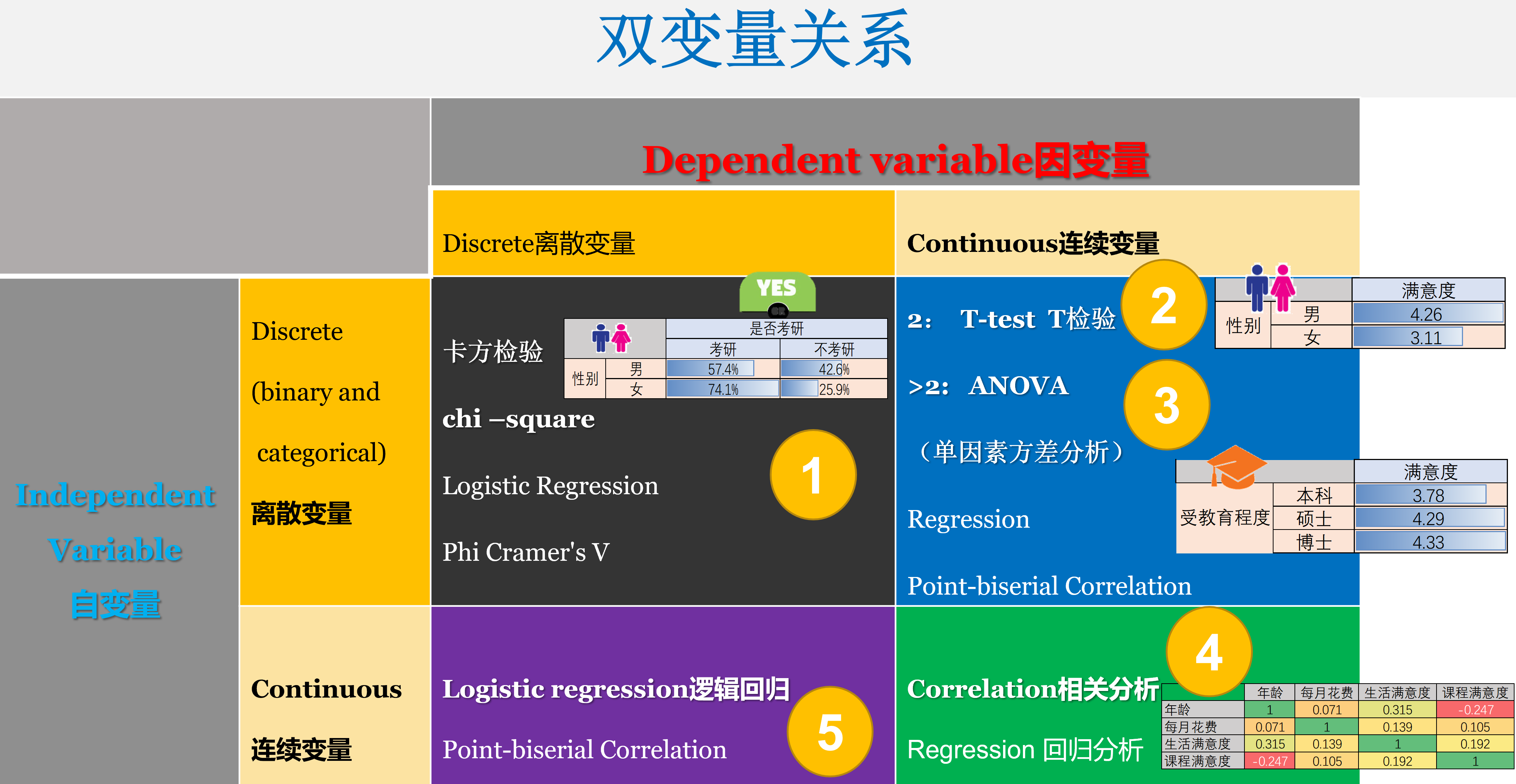
两个变量之间的关系relationship between two variables
types of variables (level of measurment)
https://statistics.laerd.com/statistical-guides/types-of-variable.php
https://www.thoughtco.com/independent-and-dependent-variable-examples-606828
https://datatab.net/tutorial/level-of-measurement
数据准备data preparation (data cleaning or data wrangling)
3.1 频数分析frequency Analysis(分类变量)
https://libguides.library.kent.edu/SPSS/FrequenciesCategorical
https://www.spss-tutorials.com/spss-frequencies-command/
https://datatab.net/tutorial/frequency-table
中文参考
https://zhuanlan.zhihu.com/p/108860781
3.2 列联表分析cross-table(分类变量)
https://libguides.library.kent.edu/SPSS/Crosstabs
中文参考
https://zhuanlan.zhihu.com/p/634975678
3.3 描述性统计分析Descriptive analysis(数值变量)
https://libguides.library.kent.edu/SPSS/Descriptives
https://www.spss-tutorials.com/spss-descriptives-command/
中文参考
https://blog.csdn.net/qq_42278015/article/details/119696576
4.1 卡方检验chi-square test
https://libguides.library.kent.edu/SPSS/ChiSquare
https://datatab.net/tutorial/chi-square-test
4.2 独立样本T检验independent sample t-test
https://libguides.library.kent.edu/SPSS/IndependentTTest
https://datatab.net/tutorial/unpaired-t-test
中文参考
https://blog.csdn.net/qq_51843109/article/details/123612791
4.3 单因素方差分析ANOVA
https://libguides.library.kent.edu/SPSS/OneWayANOVA
https://datatab.net/tutorial/anova
中文参考
https://zhuanlan.zhihu.com/p/448983174
4.4 相关分析correlation
https://libguides.library.kent.edu/SPSS/PearsonCorr
https://datatab.net/tutorial/correlation
中文参考
https://blog.csdn.net/nekonekoboom/article/details/116708114
4.5 逻辑回归分析logistic regression
https://www.spss-tutorials.com/logistic-regression/
https://datatab.net/tutorial/logistic-regression
中文参考
https://zhuanlan.zhihu.com/p/340480145
5.量表分析analysis for scales (measurement)
5.1 信度分析reliability analysis
https://www.spss-tutorials.com/cronbachs-alpha-in-spss/
https://www.spss-tutorials.com/spss-split-half-reliability/
https://datatab.net/tutorial/cronbachs-alpha
中文参考
https://www.zhihu.com/tardis/zm/art/270005975
5.2 探索性因子分析(用于效度分析)exploratory factor analysis (EFA)
https://www.spss-tutorials.com/spss-factor-analysis-tutorial/
https://www.spss-tutorials.com/spss-factor-analysis-intermediate-tutorial/
https://www.spss-tutorials.com/apa-reporting-factor-analysis/
https://datatab.net/tutorial/exploratory-factor-analysis
中文参考
https://www.zhihu.com/tardis/zm/art/270005975
6.输出分析结果export result
https://www.spss-tutorials.com/spss-output/
https://www.spss-tutorials.com/spss-apa-format-descriptives-tables/
中文参考
https://spss.mairuan.com/jiqiao/spss-wuxja.html
 http://kaiwu.city/openfiles/academic_report_SPSS_CN.docx
- 文章信息
- 作者: kaiwu
- 点击数:153
simulated dataset (tourist satisfaction)
1. questionnaire
http://kaiwu.city/openfiles/tourist_satisfaction_questionnaire_en.docx
![]() http://kaiwu.city/openfiles/tourist_satisfaction_questionnaire_en.pdf
http://kaiwu.city/openfiles/tourist_satisfaction_questionnaire_en.pdf
| No. | variable | variable labels |
| 1 | sid | Respondent ID |
| 2 | gender | gender |
| 3 | byear | Year of birth |
| 4 | region | region |
| 5 | income | monthly income |
| 6 | expense | daily expense |
| 7 | type3 | Destination type: nature, culture and mix |
| 8 | type2 | Destination type: sightseeing vs. participation |
| 9 | thotel | Types of hotel |
| 10 | sat1 | satisfaction: scenery |
| 11 | sat2 | satisfaction: hotel |
| 12 | sat3 | satisfaction: food |
| 13 | sat4 | satisfaction: transportation |
| 14 | sat5 | satisfaction: travel agency |
| 15 | sat6 | satisfaction: shopping |
| 16 | ri1 | Importance: amount |
| 17 | ri2 | Importance: publishing date |
| 18 | ri3 | Importance: relevance |
| 19 | ri4 | Importance: positive |
| 20 | ri5 | Importance: credibility |
| 21 | rp1 | Performance: amount |
| 22 | rp2 | Performance: publishing date |
| 23 | rp3 | Performance: relevance |
| 24 | rp4 | Performance: positive |
| 25 | rp5 | Performance: credibility |
| 26 | te1 | thrill |
| 27 | te2 | indulgence |
| 28 | te3 | enjoyment |
| 29 | te4 | excitement |
| 30 | te5 | liberaty |
| 31 | te6 | freedom |
| 32 | te7 | refreshment |
| 33 | te8 | revitalization |
| 34 | zh1 | uncomfortable when there are many people |
| 35 | zh2 | I dislike interpersonal communication |
| 36 | zh3 | I’m not good at interpersonal communication |
| 37 | zh4 | I try to avoid face-to-face communication |
| 38 | zh5 | Going out is a tiring thing for me. |
| 39 | zh6 | I try to avoid going out |
| 40 | zh7 | It’s troublesome for me to go out. |
| 41 | latitude | latitude |
| 42 | longitude | longitude |
| value labels | |
| Value labels gender | |
| 1 | male |
| 2 | female. |
| Value labels region | |
| 1 | Central China |
| 2 | East China |
| 3 | North China |
| 4 | Northeast China |
| 5 | Northwest China |
| 6 | Southwest China |
| 7 | West China. |
| Value labels type3 | |
| 1 | natural scenery |
| 2 | historical scenery |
| 3 | mixed scenery. |
| Value labels type2 | |
| 1 | sightseeing |
| 2 | participation. |
| Value labels thotel | |
| 1 | budget hotel |
| 2 | luxury hotel |
| 3 | bed and breakfast |
| 4 | apartment hotel. |
2. dataset
2.1 csv file
general purpose (without variable labels and value labels)
http://kaiwu.city/openfiles/tourist.csv
or
2.2 Excel file
http://kaiwu.city/openfiles/data_tourist_satisfaction_en.xlsx
or
2.3 SPSS file
http://kaiwu.city/openfiles/data_tourist_satisfaction_en.sav
3. python ipynb file
![]() http://kaiwu.city/openfiles/tourist_EN2024Nov10.ipynb
http://kaiwu.city/openfiles/tourist_EN2024Nov10.ipynb
4.results
http://kaiwu.city/openfiles/academic_report_SPSS_EN.docx
3.1 frequency Analysis(discrete variables)
https://libguides.library.kent.edu/SPSS/FrequenciesCategorical
https://www.spss-tutorials.com/spss-frequencies-command/
https://datatab.net/tutorial/frequency-table
3.2 cross-table(discrete variables)
https://libguides.library.kent.edu/SPSS/Crosstabs
3.3 Descriptive analysis(continuous variables)
https://libguides.library.kent.edu/SPSS/Descriptives
https://www.spss-tutorials.com/spss-descriptives-command/
3.4 custom table
https://www.ibm.com/docs/en/spss-statistics/saas?topic=statistics-custom-tables
http://kaiwu.city/index.php/spss-custom-table
4.relationship between two variables
types of variables (level of measurment)
https://statistics.laerd.com/statistical-guides/types-of-variable.php
https://www.thoughtco.com/independent-and-dependent-variable-examples-606828
https://datatab.net/tutorial/level-of-measurement
4.1 chi-square test
https://libguides.library.kent.edu/SPSS/ChiSquare
https://datatab.net/tutorial/chi-square-test
4.2 independent sample t-test
https://libguides.library.kent.edu/SPSS/IndependentTTest
https://datatab.net/tutorial/unpaired-t-test
4.3 ANOVA
https://libguides.library.kent.edu/SPSS/OneWayANOVA
https://datatab.net/tutorial/anova
4.4 correlation
https://libguides.library.kent.edu/SPSS/PearsonCorr
https://datatab.net/tutorial/correlation
4.5 logistic regression
https://www.spss-tutorials.com/logistic-regression/
https://datatab.net/tutorial/logistic-regression
5.analysis for scales (measurement)
5.1 reliability analysis
https://www.spss-tutorials.com/cronbachs-alpha-in-spss/
https://www.spss-tutorials.com/spss-split-half-reliability/
https://datatab.net/tutorial/cronbachs-alpha
5.2 exploratory factor analysis (EFA) for validity analysis
https://www.spss-tutorials.com/spss-factor-analysis-tutorial/
https://www.spss-tutorials.com/spss-factor-analysis-intermediate-tutorial/
https://www.spss-tutorials.com/apa-reporting-factor-analysis/
https://datatab.net/tutorial/exploratory-factor-analysis
6.export result
https://www.spss-tutorials.com/spss-output/
https://www.spss-tutorials.com/spss-apa-format-descriptives-tables/
- 文章信息
- 作者: kaiwu
- 点击数:625
![]() http://kaiwu.city/openfiles/tourist_satisfaction_questionnaire_cn.pdf
http://kaiwu.city/openfiles/tourist_satisfaction_questionnaire_cn.pdf
1.python基础
python介绍
http://kaiwu.city/index.php/python
python推荐书籍
http://kaiwu.city/index.php/python-book
2.python软件的安装
http://kaiwu.city/index.php/python-vscode
http://kaiwu.city/openfiles/python-3.13.0-amd64.exe
http://kaiwu.city/openfiles/tourist.zip
3.使用python控制Excel
http://kaiwu.city/openfiles/hotel50python.xlsx
![]() http://kaiwu.city/openfiles/python_excel50hotel.ipynb
http://kaiwu.city/openfiles/python_excel50hotel.ipynb